Introduction
In 1961, meteorologist Edward Lorenz made an accidental discovery that would revolutionize our understanding of prediction and determinism. Running a weather simulation, he rounded initial conditions from six decimal places to three. The resulting forecast diverged dramatically from his previous run—tiny differences exploded into completely different weather patterns. This observation, along with subsequent mathematical investigations, launched chaos theory and fundamentally altered how we view complex systems from weather to ecosystems to economics.
Chaos theory reveals a profound paradox: simple, deterministic systems—governed by precise mathematical laws with no randomness—can nevertheless produce behavior so complex and sensitive to initial conditions that long-term prediction becomes practically impossible. This isn’t a limitation of our measurement tools or computational power (though those matter too). It’s a fundamental property of certain nonlinear systems where small causes produce large effects.
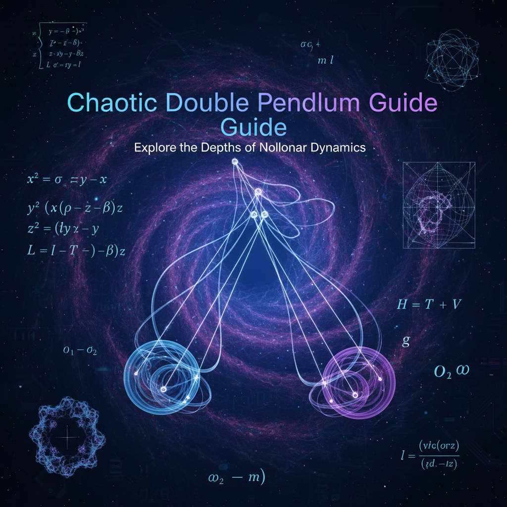
The double pendulum stands as chaos theory’s iconic demonstration. Take a simple pendulum—a mass hanging from a string—and its motion is perfectly predictable, swinging back and forth in regular periodic patterns. Add just one additional joint, creating two connected pendulums, and the system transforms into a showcase of chaos. The Chaotic Double Pendulum simulator brings this phenomenon to life, allowing anyone to witness how deterministic laws produce unpredictable complexity.
Understanding chaos theory matters far beyond abstract mathematics. Weather forecasting, climate modeling, population dynamics, neural networks, financial markets, and even the solar system’s long-term evolution all exhibit chaotic behavior. Recognizing when systems are chaotic helps us understand the limits of prediction, design better control strategies, and appreciate the delicate balance between order and disorder that characterizes much of nature.
This comprehensive guide explores the mathematics, physics, and philosophy of chaos through the lens of the double pendulum. We’ll examine what makes systems chaotic, how chaos differs from randomness, methods for analyzing chaotic behavior, and the profound implications of deterministic unpredictability for science and society.
Background: The Mathematics and Physics of Chaos
Defining Chaos: Three Essential Characteristics
Mathematicians use the term “chaos” precisely, not as a synonym for disorder or randomness. A chaotic system exhibits three key properties:
1. Deterministic: The system follows exact mathematical rules with no random elements. Given identical initial conditions, the system evolves identically every time. This distinguishes chaos from stochastic (random) processes.
2. Sensitive Dependence on Initial Conditions: Trajectories starting arbitrarily close together diverge exponentially over time. This sensitivity means tiny measurement imprecisions or rounding errors amplify until predictions become worthless. Edward Lorenz famously described this as the “butterfly effect”—the flap of a butterfly’s wings in Brazil theoretically influencing tornado formation in Texas weeks later.
3. Topological Mixing: The system’s evolution mixes regions of state space, so trajectories starting in one region eventually visit all accessible regions. This property ensures chaotic motion explores the full range of possible behaviors rather than settling into simple patterns.
Systems lacking any of these properties aren’t technically chaotic. Simple periodic motion (like a pendulum swinging regularly) is deterministic but not sensitive to initial conditions. Random noise shows sensitivity but isn’t deterministic. True chaos requires all three characteristics simultaneously.
The Double Pendulum: Equations of Motion
A double pendulum consists of two point masses connected by massless rigid rods, with the first rod pivoting from a fixed point. The system has two degrees of freedom—the angles θ₁ and θ₂ of each segment measured from vertical. The Lagrangian formulation of classical mechanics yields coupled nonlinear differential equations describing the motion:
The equations involve products and sums of trigonometric functions of the angle difference (θ₁ - θ₂), creating nonlinear coupling between the two segments. This nonlinearity is the mathematical source of chaos—linear systems cannot exhibit chaotic behavior.
For small angles and weak coupling, perturbation methods yield approximate solutions. But for large angles (which the system naturally explores), no analytical solution exists. We must solve the equations numerically using methods like Runge-Kutta integration—essentially simulating the system’s evolution step by step through time.
The Chaotic Double Pendulum simulator implements these equations with high numerical precision, allowing users to explore chaotic dynamics without deriving or solving the mathematics themselves.
Energy Conservation and Phase Space
Despite complex motion, the double pendulum conserves total mechanical energy in the absence of friction. Kinetic energy (from motion) and potential energy (from height in a gravitational field) continuously exchange, with their sum remaining constant. This conservation law constrains possible motions—the system can only access states with matching total energy.
Phase space provides a powerful framework for visualizing dynamical systems. For the double pendulum, we can plot a four-dimensional space with coordinates (θ₁, θ₂, ω₁, ω₂) representing both angles and angular velocities. Each point in this space represents one possible system state, and system evolution traces a trajectory through phase space.
Energy conservation means trajectories lie on a three-dimensional surface (a “manifold”) within the four-dimensional phase space. Chaotic trajectories wander across this energy surface in complex, never-repeating patterns. In contrast, simple periodic motion traces closed loops in phase space—same states revisited repeatedly.
Poincaré sections simplify visualization by sampling the trajectory when it crosses a specific plane (e.g., when θ₁ = 0 while moving in a particular direction). These points form patterns called strange attractors for chaotic systems—fractal structures with non-integer dimensions that reveal the underlying organization within apparent chaos.
Lyapunov Exponents: Quantifying Chaos
How can we measure “how chaotic” a system is? Lyapunov exponents provide a quantitative answer by measuring the average exponential rate at which nearby trajectories diverge.
Start two trajectories with initial separation δ₀. After time t, their separation grows approximately as δ(t) ≈ δ₀ exp(λt), where λ is the Lyapunov exponent. Positive λ indicates exponential divergence (chaos), λ ≈ 0 indicates neutral stability, and negative λ indicates convergence.
For systems with multiple degrees of freedom, there are multiple Lyapunov exponents (as many as dimensions). A system is chaotic if its largest Lyapunov exponent is positive. The double pendulum typically has one positive, one near-zero, and two negative Lyapunov exponents depending on parameter choices.
The reciprocal of the largest Lyapunov exponent gives a timescale for prediction—roughly how long until forecasts become unreliable. For Earth’s atmosphere, this Lyapunov timescale is about 2 weeks, explaining why weather forecasts beyond 10-14 days have little skill.
Historical Development: From Poincaré to Modern Chaos Theory
While Edward Lorenz’s 1961 discovery catalyzed modern interest, chaos theory’s roots extend deeper. Henri Poincaré, investigating the three-body problem in celestial mechanics (1880s-1890s), discovered that tiny perturbations to planetary orbits could produce large effects over long timescales. He realized the solar system’s long-term evolution might be fundamentally unpredictable—a revolutionary insight given Newtonian determinism’s philosophical dominance.
The mid-20th century saw renewed mathematical interest in nonlinear dynamics. Russian mathematicians Kolmogorov, Arnold, and Moser developed the KAM theorem describing the transition from integrable (solvable) systems to chaotic ones. American mathematicians like Stephen Smale studied structural stability and strange attractors.
Lorenz’s work brought chaos theory to broader scientific attention, especially when computer visualization made abstract mathematics tangible. Benoit Mandelbrot’s fractal geometry revealed chaotic systems’ hidden order. Mitchell Feigenbaum discovered universal constants governing the transition to chaos through period-doubling bifurcations.
By the 1980s, chaos theory pervaded scientific disciplines. Biologists modeled population dynamics, economists studied market fluctuations, engineers analyzed fluid turbulence, and physicists investigated quantum chaos. The double pendulum became an educational icon because it demonstrates sophisticated mathematical concepts through a simple mechanical system anyone can understand.
Workflows: Exploring Chaos Through Simulation
Beginner Workflow: Experiencing Sensitive Dependence
Step 1: Launch and Observe
Open the Chaotic Double Pendulum simulator. Set both segments to moderate angles (around 60 degrees from vertical) and release. Watch the complex, unpredictable motion for 30-60 seconds. Notice that the motion never settles into a regular pattern—it continuously explores new configurations.
Step 2: Test Reproducibility (Determinism)
Reset the simulation and launch from the same initial position. Observe that the trajectory repeats exactly—this demonstrates determinism. The system isn’t random; it follows precise physical laws.
Step 3: Introduce Tiny Differences (Sensitivity)
Enable comparison mode. Launch two pendulums: one at θ₁ = 60.000° and another at θ₁ = 60.001° (a difference of 0.001°, far smaller than you could measure with a protractor). Initially, both move nearly identically. After several seconds, their paths diverge noticeably. After 10-20 seconds, they bear no resemblance despite having started from nearly identical conditions. This demonstrates sensitive dependence on initial conditions.
Step 4: Contrast with Simple Pendulum
Open the Interactive Pendulum Lab in another browser tab. Launch a simple pendulum from 60°. It swings predictably back and forth. Launch two simple pendulums with 60.000° and 60.001°—their motions remain nearly identical indefinitely. This contrast illustrates that adding one degree of freedom (second pendulum segment) transforms predictable dynamics into chaos.
Intermediate Workflow: Parameter Exploration
Phase 1: Mass Ratio Effects
Systematically vary the ratio of upper to lower mass while keeping lengths equal. Try ratios of 0.1, 0.5, 1.0, 2.0, and 10.0. For each configuration, launch pairs with 0.001° initial difference and measure time until trajectories diverge by 10° (your operational definition of “significantly different”). You’ll likely find equal masses (ratio = 1.0) produce fastest divergence (strongest chaos), while extreme mass ratios reduce chaotic intensity.
Phase 2: Length Configuration Studies
Investigate how segment lengths affect behavior. Equal lengths produce symmetric motion initially breaking into complex patterns. Very long lower segments with short upper segments create distinct motion character from the reverse configuration. Document which geometries produce most visually striking patterns.
Phase 3: Energy and Damping
With zero damping, total energy remains constant and motion continues indefinitely. Add slight damping (air resistance coefficient around 0.02) and watch energy gradually dissipate. Notice that chaotic behavior persists even as amplitude decays—chaos doesn’t require large swings. Eventually, the pendulum settles to hanging vertically (a stable equilibrium point).
Phase 4: Initial Condition Surveys
Create a grid of initial conditions varying both θ₁ and θ₂ from 0° to 180° in 15° increments. For each, observe whether motion remains relatively simple or becomes highly chaotic. You might discover that small initial displacements tend toward more regular motion while large angles promote chaos—though exceptions abound, reflecting the complexity of the system.
Advanced Workflow: Quantitative Chaos Analysis
Lyapunov Exponent Estimation
Calculate the largest Lyapunov exponent numerically:
- Launch two simulations with initial separation δ₀ = 0.0001 radians
- Let both evolve for time Δt = 0.1 seconds
- Measure separation δ(Δt) in phase space (distance considering both position and velocity differences)
- Renormalize: move one trajectory to maintain fixed separation δ₀ while preserving direction
- Repeat for many iterations, accumulating the logarithm of growth factors
- Average: λ ≈ (1/T) Σ ln(δᵢ/δ₀) over total time T
Positive λ confirms chaos; larger values indicate stronger sensitivity.
Phase Space Visualization
Export trajectory data and plot in three-dimensional space using coordinates like (θ₁, θ₂, ω₁). The trajectory traces a complex curve never exactly repeating. Compare this with a simple pendulum’s phase space trajectory (a closed ellipse) to appreciate the difference between integrable and chaotic systems.
Poincaré Section Analysis
Sample the trajectory whenever it crosses a specific surface (e.g., θ₁ = 0 with positive ω₁). Plot these crossing points in (θ₂, ω₂) space. For chaotic motion, points form fractal patterns (strange attractors). For periodic motion, points cluster at discrete locations. For quasi-periodic motion, points trace closed curves.
Fourier Analysis
Compute the frequency spectrum of angular position θ₁(t) using Fast Fourier Transform. Simple periodic motion shows discrete frequency peaks. Chaotic motion displays broadband spectra—energy distributed across many frequencies rather than concentrated at a fundamental and harmonics.
Educational Workflow for Classroom Integration
Pre-Lesson Preparation
Before introducing chaos theory formally, have students explore the Chaotic Double Pendulum freely. Ask them to describe what they observe in their own words. Common responses: “random,” “unpredictable,” “messy,” “complex.” This unstructured exploration primes students for formal concepts.
Guided Discovery Activity
Provide worksheets with specific investigations:
- “Launch from θ₁ = 90°, θ₂ = 0°. Sketch the path of the lower mass for 10 seconds.”
- “Launch two pendulums with angles differing by 0.01°. At what time do they first differ by more than 10° in any coordinate?”
- “Compare motion with equal masses (1 kg each) versus unequal (2 kg upper, 0.5 kg lower). Describe differences qualitatively.”
Class Discussion and Synthesis
After data collection, facilitate discussion where students share findings. Introduce formal terminology: deterministic, sensitive dependence, chaotic. Show how their observations exemplify these concepts. Contrast with the Interactive Pendulum Lab simple pendulum to highlight the transition from integrable to chaotic systems.
Extension Projects
Advanced students can:
- Research real-world chaotic systems (weather, heart rhythms, stock markets) and present findings
- Estimate Lyapunov exponents using exported data
- Explore the Physics Simulation Lab three-body problem as another chaotic system
- Read popularizations like James Gleick’s “Chaos: Making a New Science” for historical context
Comparisons: Chaotic vs. Non-Chaotic Systems
Simple Pendulum (Non-Chaotic) vs. Double Pendulum (Chaotic)
The contrast between simple and double pendulums illuminates what chaos means:
Simple Pendulum Characteristics:
- One degree of freedom (single angle variable)
- Linear restoring force for small angles: F ∝ -θ
- Periodic motion: same positions revisited regularly
- Period depends only on length and gravity: T = 2π√(L/g)
- Nearby trajectories remain close indefinitely (stable motion)
- Phase space trajectory is a closed ellipse
- Completely predictable over all timescales
Double Pendulum Characteristics:
- Two degrees of freedom (two angle variables)
- Nonlinear coupling between segments
- Aperiodic motion: never exactly repeats
- No simple formula for period or trajectory
- Nearby trajectories diverge exponentially (chaotic motion)
- Phase space trajectory is a complex fractal (strange attractor)
- Practically unpredictable beyond short timescales
Adding just one degree of freedom and introducing nonlinear coupling transforms the system fundamentally. This illustrates a general principle: complexity and chaos often emerge from interactions between simple components rather than from individual component complexity.
Deterministic Chaos vs. Randomness
Chaos and randomness are frequently confused but represent fundamentally different phenomena:
Deterministic Chaos:
- Governed by precise mathematical equations
- Identical initial conditions produce identical outcomes
- Unpredictability arises from sensitivity, not intrinsic randomness
- Contains hidden structure (strange attractors, fractal patterns)
- Can be simulated with complete reproducibility
- Example: Double pendulum, weather systems, turbulent fluids
True Randomness:
- No underlying deterministic rule governs outcomes
- Identical initial conditions can produce different outcomes
- Unpredictability is fundamental, not merely practical
- No structured patterns—purely stochastic
- Cannot be simulated exactly, only sampled from probability distributions
- Example: Quantum measurements, radioactive decay, ideal dice rolls
Philosophically, this distinction matters enormously. Chaos preserves determinism—the universe follows laws—while acknowledging practical limits to prediction. Randomness introduces fundamental indeterminism. The double pendulum is chaotic (deterministic) not random.
Periodic, Quasi-Periodic, and Chaotic Motion
Dynamical systems exhibit several distinct behaviors:
Periodic Motion:
- Trajectory repeats exactly after fixed time interval (period)
- Phase space: closed loops
- Frequency spectrum: discrete peaks
- Lyapunov exponent: zero or negative
- Example: Simple pendulum, planetary orbits (approximately)
Quasi-Periodic Motion:
- Trajectory combines multiple incommensurate frequencies
- Never exactly repeats but remains bounded and structured
- Phase space: trajectories lie on tori (donut shapes)
- Frequency spectrum: multiple discrete peaks
- Lyapunov exponent: zero
- Example: Two coupled oscillators with irrational frequency ratio
Chaotic Motion:
- Aperiodic—never repeats exactly
- Sensitive to initial conditions
- Phase space: strange attractors with fractal structure
- Frequency spectrum: broadband (continuous)
- Lyapunov exponent: positive
- Example: Double pendulum (typically), atmospheric convection, turbulence
Systems can transition between these behaviors as parameters change. For instance, progressively increasing the energy of a double pendulum might transition from periodic (low energy, small angles) through quasi-periodic to fully chaotic (high energy, large angles).
Best Practices for Understanding and Working with Chaotic Systems
Conceptual Understanding Strategies
Embrace Uncertainty: Recognize that unpredictability doesn’t mean ignorance or poor modeling. Chaos represents a fundamental limit to prediction, not a temporary obstacle awaiting better technology. Weather forecasts will never be accurate 30 days out, regardless of computational power, because the atmosphere is chaotic.
Distinguish Determinism from Predictability: Deterministic systems follow exact laws, but this doesn’t guarantee predictability. The double pendulum’s equations are perfectly known, yet we cannot forecast its position far into the future. Accepting this paradox is essential for understanding chaos.
Appreciate Timescales: Chaotic systems are predictable in the short term but not the long term. Weather forecasts are skillful for 3-7 days, mediocre for 7-10 days, and useless beyond 14 days. Understanding relevant timescales (related to Lyapunov exponents) helps set appropriate expectations.
Recognize Order Within Chaos: Chaotic systems aren’t completely random. They exhibit structured patterns—strange attractors, fractal dimensions, statistical regularities. We can often predict statistical properties (average behaviors) even when specific trajectories elude prediction.
Simulation and Analysis Best Practices
Use Appropriate Numerical Methods: Chaotic systems amplify numerical errors, so high-accuracy integration methods (Runge-Kutta 4th order or higher) are essential. The Chaotic Double Pendulum simulator uses RK4 integration precisely for this reason.
Verify Energy Conservation: In frictionless simulations, total energy should remain constant. If energy drifts over time, numerical integration timestep may be too large, causing errors. This provides a sanity check on simulation accuracy.
Run Ensemble Simulations: Since individual trajectories are unpredictable, run many simulations with slightly different initial conditions. Statistical properties of the ensemble (average behavior, probability distributions) often reveal meaningful patterns invisible in single realizations.
Document Everything: When exploring chaotic systems, meticulously record all parameters, initial conditions, and observations. Reproducing interesting behaviors later is impossible without exact documentation since tiny parameter changes produce different outcomes.
Start Simple, Add Complexity Gradually: Begin investigations with simplified scenarios (small angles, equal masses, no damping). Build understanding of basic behavior before introducing realistic complications (large angles, damping, unequal masses).
Teaching and Learning Strategies
Use Interactive Tools: Static diagrams and equations cannot convey chaos’s dynamic nature. Interactive simulations like the Chaotic Double Pendulum make abstract concepts tangible through direct manipulation and observation.
Emphasize Exploration: Chaos theory resists passive learning. Students must experiment—launching simulations with various parameters, comparing outcomes, discovering patterns themselves. This active engagement builds intuition textbooks cannot provide.
Connect to Real-World Examples: Abstract mathematical chaos becomes meaningful when linked to weather prediction, ecosystem dynamics, economic markets, or heart arrhythmias. These connections motivate deeper study and demonstrate relevance beyond theoretical interest.
Address Philosophical Implications: Chaos theory challenges naïve determinism (knowing laws and initial conditions doesn’t guarantee prediction) and raises questions about free will, complexity, and the limits of science. Thoughtful discussion of these themes enriches understanding.
Provide Multiple Representations: Use visualizations (phase space plots, time series, Poincaré sections), equations, simulations, and verbal explanations. Different students connect with different representations; multiple modalities reinforce understanding.
Case Study: Chaos in the Solar System
The Stability Question
For centuries, astronomers wondered whether the solar system is stable over astronomically long timescales. Newton’s laws determine planetary motion precisely—a deterministic system. Early celestial mechanics (Laplace, Lagrange) proved stability for simplified models (two-body problems, averaging methods). But the full N-body problem with mutual gravitational interactions remained unsolved.
Henri Poincaré demonstrated in the 1880s that the three-body problem (Sun, Earth, Moon, for instance) has no general analytical solution and exhibits sensitive dependence on initial conditions—chaos. This raised disturbing questions: Could tiny perturbations eventually destabilize planetary orbits? Might Earth get ejected from the solar system or collide with Venus?
Modern Computational Investigations
Late 20th-century computers enabled numerical integration of planetary orbits over millions of years. Researchers discovered:
Inner Solar System Chaos: Orbits of Mercury, Venus, Earth, and Mars exhibit chaotic behavior with Lyapunov timescales of approximately 5 million years. This doesn’t mean orbits change drastically in 5 million years, but small uncertainties in current positions amplify until detailed trajectory prediction becomes meaningless beyond that timeframe.
Long-Term Instability Probability: Integrations over billions of years show small but non-zero probability of orbital instability. Mercury has roughly 1% chance of becoming unstable within the Sun’s remaining lifetime (5 billion years), potentially causing collisions or ejections.
Resonances and Protection: Despite chaos, the solar system exhibits remarkable stability due to orbital resonances and angular momentum conservation. Chaos explores possibilities within constraints—orbits wander within bounds rather than flying to extremes.
Philosophical Implications
The solar system’s chaos illustrates several profound insights:
Limits of Determinism: We know Newton’s laws exactly. We’ve measured planetary positions precisely. Yet we cannot predict where Mercury will be in 100 million years with confidence. The future, though determined by laws, remains fundamentally uncertain beyond timescales set by Lyapunov exponents.
Historical Contingency: Small differences in the early solar system’s formation (tiny variations in dust cloud turbulence) could have produced dramatically different planetary configurations today. Our solar system’s specific arrangement may be partly accidental rather than inevitable.
Probability in Deterministic Systems: Though individually deterministic, chaotic trajectories can be described statistically. We cannot say where Mercury will be in 100 million years, but we can estimate probabilities for different orbital elements. This probabilistic description emerges from deterministic chaos, not quantum uncertainty.
The solar system’s chaos mirrors the double pendulum’s lessons. Simple deterministic rules (gravity, Newton’s laws) plus nonlinear interactions (mutual planetary perturbations) produce complex, ultimately unpredictable behavior—orderly chaos that shapes cosmic evolution over eons.
Call to Action
Chaos theory fundamentally changes how we understand prediction, determinism, and complexity. The Chaotic Double Pendulum provides an accessible entry point into this fascinating domain where simple systems reveal unexpected depths.
For Students: Don’t just read about chaos—experience it directly. Launch simulations, make predictions, observe how tiny changes cascade into large effects. This hands-on exploration builds intuition that equations alone cannot provide. Complement the double pendulum with related tools like the Interactive Pendulum Lab to appreciate the contrast between simple and chaotic systems.
For Educators: Chaos theory offers rich opportunities for inquiry-based learning. Design investigations where students discover sensitivity to initial conditions themselves rather than being told about it. Connect mathematical abstractions to tangible phenomena—weather forecasting, ecosystem dynamics, heart arrhythmias—to demonstrate relevance and inspire curiosity.
For Researchers: Chaos appears across scientific disciplines. Whether studying fluid turbulence, neural networks, economic systems, or climate dynamics, understanding chaotic behavior is essential. Use tools like the Physics Simulation Lab for pedagogical foundations, then advance to specialized software for research applications.
For Philosophers and Curious Minds: Chaos theory raises profound questions about determinism, free will, complexity, and the nature of scientific knowledge. How do we make decisions in chaotic systems where long-term prediction is impossible? What does chaos mean for our ability to control complex systems? These questions extend far beyond physics into ethics, policy, and human understanding.
Explore the Chaotic Double Pendulum today. Watch order emerge from determinism, beauty from complexity, and humility from the recognition that knowing the laws doesn’t mean we can predict the future. Chaos invites us to embrace uncertainty while still searching for understanding—a powerful lesson extending far beyond physics into how we navigate our complex, unpredictable world.
References and Further Reading
-
Lorenz, E. N. (1963). Deterministic nonperiodic flow. Journal of the Atmospheric Sciences, 20(2), 130-141. https://doi.org/10.1175/1520-0469(1963)020<0130:DNF>2.0.CO;2 [The foundational paper describing the Lorenz attractor and establishing meteorological chaos]
-
Strogatz, S. H. (2015). Nonlinear Dynamics and Chaos: With Applications to Physics, Biology, Chemistry, and Engineering (2nd ed.). Westview Press. [Excellent textbook covering chaos theory with accessible explanations, examples, and problem sets]
-
Gleick, J. (1987). Chaos: Making a New Science. Viking Books. [Highly readable popular science book chronicling chaos theory’s development and key researchers]
-
Ott, E. (2002). Chaos in Dynamical Systems (2nd ed.). Cambridge University Press. [Comprehensive advanced treatment of chaotic dynamics for graduate students and researchers]
-
Poincaré, H. (1892-1899). Les Méthodes Nouvelles de la Mécanique Céleste (3 volumes). Gauthier-Villars. [Historic work where Poincaré discovered sensitive dependence in celestial mechanics, presaging modern chaos theory]